Distribution fitting
Your quick start tutorial to using shiny rrisk distributions
Getting started
| NEW | Click here if you wish to create a new distribution fitting project. |
| OPEN | Open a csv-data file containing your original observations or a rrisk-dist file if you want to modify a distribution fitting project that you have created and downloaded. |
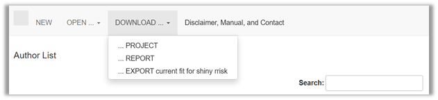
| SAVE | Download the fitting project, report or export to shiny rrisk session. |
| ABOUT | Check out here for a disclaimer, manual and contact information. |
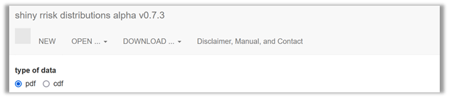
Click NEW to start a new fitting project.
Shiny rrisk distributions supports two approaches for fitting a distribution (Figure 1). The first approach allows you to fit a probability density function (pdf) to a sample of observations. The app then helps you to identify and parameterise candidate distributions that fit the provided data. The second approach involves fitting a cumulative density function (cdf), for which you will define the required percentiles. The percentiles may be generated using an expert knowledge elicitation (EKE). The percentiles are then used as support points for distribution fitting.
| Choose this option when you have original data, typically a sample from a population of observations. | |
| cdf | Choose this option when you have percentiles, e.g. from an EKE process. |
A state-of-art repertoire of methods for distribution fitting has been developed by Delignette-Muller and Dutang (2015) and is made available via the R-package fitdistrplus. The results of any external fitting routine can be used easily to define and document a distributional node in the shiny rrisk modelling framework. Using shiny rrisk distributions may be your preferred option if you are less familiar with using external resources for distribution fitting. When encountering special situations such as fitting distributions to censored data and if you need access to a broader range of validated fitting algorithms, fitdistrplus may be your choice.
In a session with this application, one distribution can be fitted at a time, which can be used to inform a distribution node in the shiny rrisk application. Consequently, each fitted distribution in shiny rrisk is documented with a corresponding distribution fitting object.
Distribution families available in shiny rrisk
Regardless of whether you choose the pdf or the cdf approach, shiny rrisk offers you a choice of discrete (?) and continuous distribution families. Note that shiny rrisk presents a preselection of distributions that are eligible according to your specifications of the pdf or cdf. See below for some guidance oselecting a distribution family.
- Discrete distributions (not yet implemented?)
- Finite support (lower and/or upper boundary)
- Bernoulli
- Binomial
- Hypergeometric
- Poisson
- Finite support (lower and/or upper boundary)
- Continuous distributions
- Finite support (with lower and/or upper boundary)
- Beta
- Exponential
- Gamma
- Inverse gamma
- Triangular
- Log-normal
- Weibull
- Infinite support
- Normal
- Cauchy
- Finite support (with lower and/or upper boundary)
Fitting a probability density function (pdf)
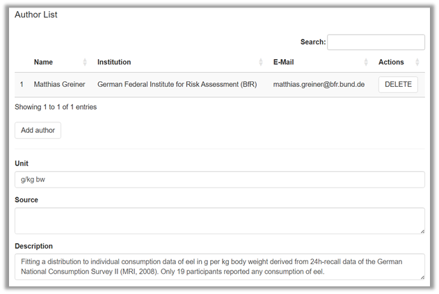
This option allows you to fit a distribution using your sample of observations. Consider as an example 19 individual consumption data of eel in g per kg body weight node that were used to inform the node X of the Alizarin red in eel model. The data can be entered data manually (Figure 2).
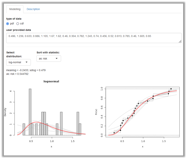
The user provided data can be entered manually as comma separated values using decimal point. The model that appears under Select distribution (here the log-normal) provides the best fit according to the selected Goodness-of-fit statistic (by default the average negative log likelihood). The fitted distribution parameters occur below. A panel with two distribution plots is shown. On the left, the entered data is shown as histogramme (grey) whereas on the right side the entered data points are shown in a cumulative distribution plot (black). In the two graphs, the selected fitted distribution is overlaid as density or distribution plot on the left and right side, respectively (red line). Other candidate distribution models are also shown (grey). You can choose alternative distributions and goodness-of-fit (GOF) statistics. Future versions of shiny distributions may provide a summary table with all candidate distributions and GOF statistics.
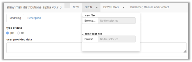
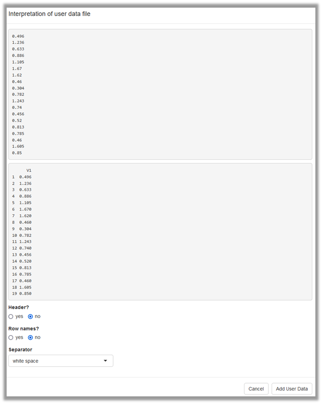
Alternatively, user provided data can be uploaded as csv file (Figure 3), which results in the same situation as the manual entry. During import of the data, you will confirm whether the data file contains column names or row names and specify the column separator (Figure 4).
General approach
There is no single commonly accepted strategy to fit a distribution to empirical data. If you are are unsure which probability density function is eligible to fit your data, you are advised to consult an expert. Consider the details provided in the Modelling framework tutorial under Building a model/ Defining a node/Parametric distributions on topics such as discrete versus continuous distributions, truncation and censoring.
Goodness-of-fit (GOF) measures
@Robert to check this definition and confirm that we are not using maximum likelihood (which would be the product rather than average L’s). Given the data set and a chosen distribution model, the average negative log likelihood (ANLL) is a GOF measure that provides the average likelihood of observing the data points given the distribution model and the optimised model parameters. The ANLL does not penalise the number of model parameters. Thus, applying this criterion for model selection may result in overfitting since distribution models with more parameters tend to fit the data points better than distributions with fewer parameters although the latter may provide a more reliable model. The Akaike information criterion (AIC) is also based on the likelihood but additionally accounts for (“penalises”) the number of model parameters. Therefore, it is generally the preferred GOF statistic (@all, should we cite wikipedia here but not elsewhere? Wikipedia contributors. ‘Akaike information criterion’, accessed 30 June 2025). Similar to AIC, the Bayesian information criterion (BIC) penalises the number of model parameters. There is a large body of scientific papers comparing AIC and BIC for model selection.
A pragmatic approach is to report all GOF statistics and use AIC or BIC for the model selection. If these statistics lead to different conclusions, the case-by-case assessment should also take into account aspects such as the model most commonly used in the scientific literature for the type of data in question and the shape properties in critical areas of the distribution, which could be the extreme values (left or right) or the mass of the distribution, depending on the problem.
Example
The exposure model of Alizarin red in eel contains the node X based on 19 observed individual intake values of eel per kg body weight derived from 24h-recall data of the German National Consumption Survey II (MRI, 2008). This model demonstrates the advanced concept of using bootstrap to obtain a joint uncertainty distribution for the log mean and log standard deviation. Here, we explore a simpler approach, which is to use the 19 original intake values directly for distribution fitting (Figure 2). A log-normal distribution provides the best fit according to the AIC statistic, which is also consistent with the BIC and ANLL results. The parameters of fitted log-normal distribution and the GOF statistics are shown above the panel with the two distribution plots.
Fitting a cumulative density function (cdf)
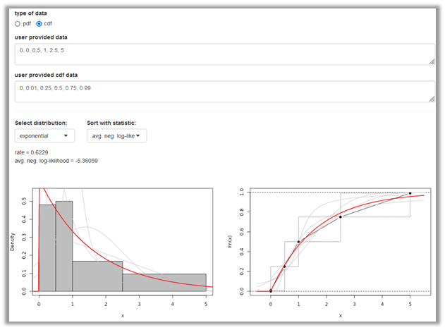
This option allows you to provide quantiles and probabilites to characterise the distribution to be fitted. (Figure 5). As example we use the node for the proportion of adults emerging from waste in percent (p_adults_emerging_from_waste) of the E.lignosellus in asparagus model. Six quantiles with corresponding probabilities have been identified to characterise the distribution based on the result of an expert knowledge elicitation (EKE) process.
@Robert: can you make the PERT eligible as candidate distribution? I cannot see how else we can accommodate EFSA’s protocol.
The User provided data are the quantiles and can be entered comma separated using decimal point. The user defined cdf data are the corresponding probabilities. Note that the quantiles and probabilities can also be uploaded as an csv data file with two columns. The interface for Select distribution (here the exponential) and Goodness-of-fit statistic are similar as shown for the pdf fitting although the underlying fitting algorithms differ between the two approaches. In the original model, a PERT model was chosen as a distribution model. @Robert, I think this is important to satisfy EFSA#s needs: Future versions of shiny distributions may include the PERT model.
@Robert: this section accounts for the fact that we have disabled the EFSA EKE option. Except the availability of the PERT for fitting a cdf everything should be fine with this simplification. I also appreciate that users may fit other distributions than PERT to their EKE results.
Using the cdf approach it is straightforward to fit a distribution to the results of a formal EKE protocol. The outcome of the EKE process for a given quantity consists of a quantile vector (user provided data), i.e. values on the scale of the quantity being modelled and a corresponding probability vector (user provided cdf data), denoting the probability that the quantity being modelled falls below the quantile value. Note that neither the quantiles nor the probabilities have to be equally spaced. Below the quantiles and probabilities are provided for the E.lignosellus in asparagus model example (Figure 5).
@Robert? Future versions of shiny distributions may allow to select a PERT as candidate distribution for fitting.
| quantile | probability |
|---|---|
| 0 | 0 |
| 0 | 0.01 |
| 0.5 | 0.25 |
| 1.0 | 0.5 |
| 2.5 | 0.75 |
| 5 | 0.99 |
@Thomas and Robert: are there any standard topics for reporting an EFSA RKE result? please edit the part below as needed (perhaps using your EFSA report).
The European Food Safety Authority (EFSA) has described a process for eliciting expert knowledge (EFSA 20XX, we need the official version here, accessed Aug 7, 2025). The use of an EFSA EKE process in shiny rrisk involves the following steps.
- Conduct EFSA EKE protocol, which includes the definition of a target quantity (description, unit, etc.) and generate the results similar to the table above.
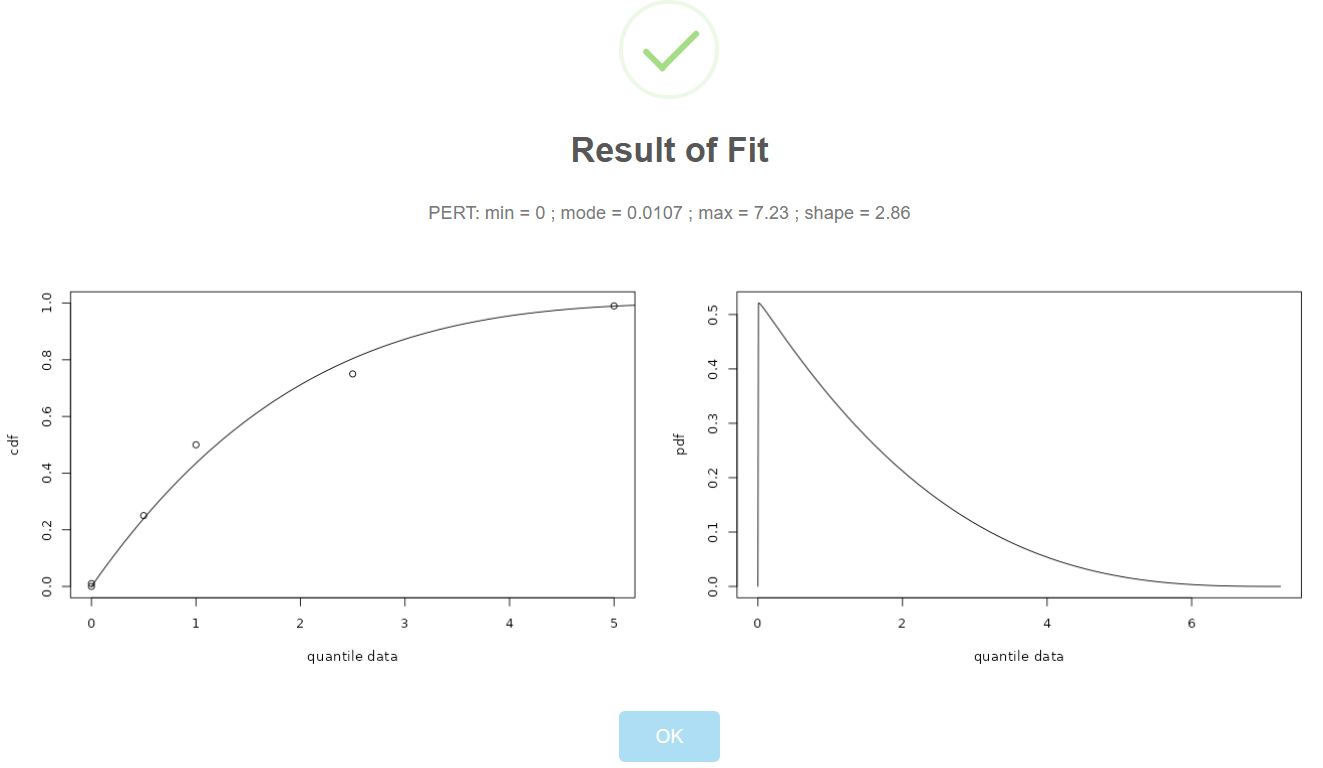
- Using shiny rrisk distributions to fit a PERT or another distribution model as described above.
- Documenting the EKE process in shiny rrisk distributions.
- Exporting the results into a shiny rrisk session (as described below).
Step 3 may involve the following subheaders that can be pasted into the description field.
# Background

# Quantity of interest

# EKE process

# Results and interpretation

# References
Expert knowledge elicitation (EKE) - old - whole section to be deleted
@Robert and Thomas to confirm that we cannpot use this section anymore.
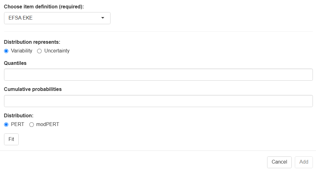
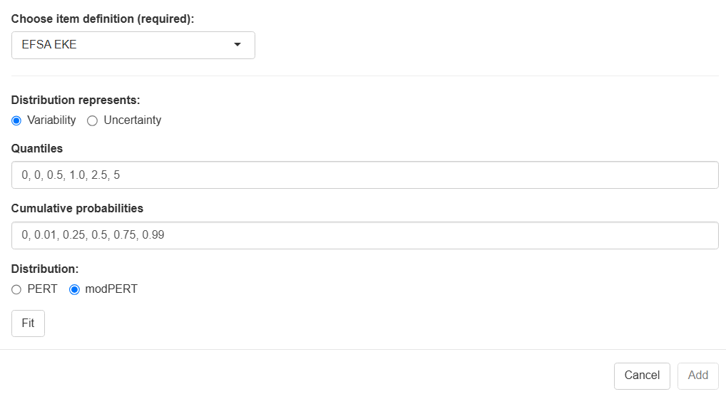
| Choose node definition | to be updated Select EFSA EKE. |
| Distribution represents | Select either variability or uncertainty. |
| Quantiles | Enter any number of quantiles, comma-separated. |
| Cumulative probability | Enter one cumulative probability for each of the quantiles, beginning with the value zero, comma-separated. |
The two steps in this example are the following.
- please complete
- …
Documentation
The documentation of the distribution fitting should be launched by choosing Description from the top row of the app (Figure 2).
@Robert: please insert a Project name entry field and Cancel & Save buttons
This opens a new window in which a documentation can be entered similar to the documentation of a shiny rrisk model (Figure 9). Technical details about the documentation are provided in the Modelling framework tutorial under Documenting and reporting | Adding general model description.
Saving your fitting results
Downloading the Project is essential for saving the fitting project and making it available for future editing (file extension “.rriskdist”). Report will launch the automatic reporting (@Robert: file extension “.docx” not yet available). Export creates an object for uploading the results into a shiny rrisk session (file extension “.rriskdistex”). This step is explained in the Modelling framework tutorial under Building a model | Defining a node | Parametric distributions.
How to cite this tutorial
Greiner M, Sanchez J, more authors (2025). Distribution fitting - your quick start tutorial to using shiny rrisk distributions. [BfR GitHub-Link], Date of last editing: September 10, 2025.